Ocultar código
library(terra)
library(glue)
library(tidyterra)
library(ggfx)
library(showtext)
library(ggtext)
library(tidyverse)Mapa de instituciones de ciencia y educación.
library(terra)
library(glue)
library(tidyterra)
library(ggfx)
library(showtext)
library(ggtext)
library(tidyverse)Colores aleatorios a partir de una gama de rosados.
c1 <- "lightblue"
c2 <- "orange"
c3 <- "white"
c4 <- "grey5"
c5 <- "grey30"
Fuentes: Ubuntu, JetBrains Mono y fontawesome.
font_add(
  family = "ubuntu",
  regular = "././fuente/Ubuntu-Regular.ttf",
  bold = "././fuente/Ubuntu-Bold.ttf",
  italic = "././fuente/Ubuntu-Italic.ttf"
)

font_add(
  family = "jet",
  regular = "././fuente/JetBrainsMonoNLNerdFontMono-Regular.ttf"
)

showtext_auto()
showtext_opts(dpi = 300)fuente <- glue(
"<b>Datos:</b> <span style='color:{c3};'>IGN</span>")
autor <- glue("<span style='color:{c3};'>Víctor Gauto</span>")
icon_twitter <- glue("<span style='font-family:jet;'></span>")
icon_instagram <- glue("<span style='font-family:jet;'></span>")
icon_github <- glue("<span style='font-family:jet;'></span>")
icon_mastodon <- glue("<span style='font-family:jet;'>󰫑</span>")
icon_bluesky <- glue("<span style='font-family:jet;'></span>")
usuario <- glue("<span style='color:{c3};'>vhgauto</span>")
sep <- glue("**|**")
mi_caption <- glue(
"{fuente} {sep} {autor} {sep} <b>{icon_github} {icon_twitter} ",
"{icon_instagram} {icon_mastodon} {icon_bluesky}</b> {usuario}"
)Obtengo los datos del Instituto Geográfico Nacional, en la categoría Ciencia y educación, Universidad.
u <- vect("argentina/vectores/puntos_de_ciencia_y_educacion_020602.json") |>
  project("EPSG:5346")
Leo los datos de las provincias y departamentos de Argentina.
dptos <- vect("argentina/vectores/dptos_continental.gpkg")
pcias <- vect("argentina/vectores/pcias_continental.gpkg")
Me interesa la Universidad Tecnológica Nacional (UTN).
d <- u |>
  mutate(
    es_utn = str_detect(gna, "Universidad Tecnológica Nacional")
  ) |>
  mutate(
    es_utn = if_else(
      is.na(es_utn),
      FALSE,
      es_utn
    )
  )
Divido los datos según si son de la UTN o del resto de instituciones.
d_utn <- filter(d, es_utn)
d_otra <- filter(d, !es_utn)
Cantidad total de UTN.
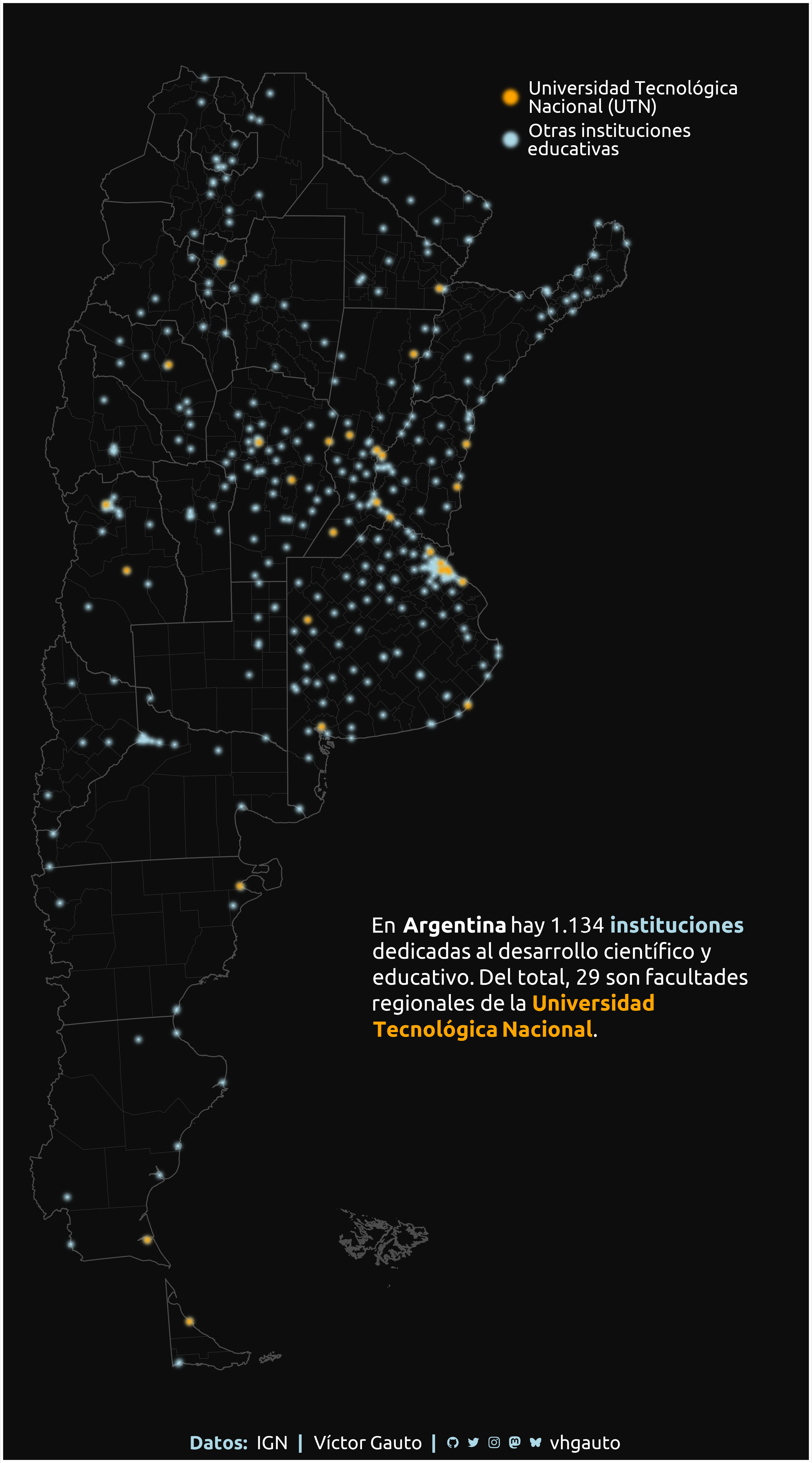
n_u <- format(nrow(u), big.mark = ".", decimal.mark = ",")Descripción y subtítulo del mapa.
leyenda_tbl <- tibble(
  x = 5.1e6,
  y = c(7.5e6, 7.38e6),
  label = c(
    "Universidad Tecnológica\nNacional (UTN)",
    "Otras instituciones\neducativas")
) |>
  mutate(x_label = x+.5e5)

mi_subtitle <- glue(
  "En <b>Argentina</b> hay {n_u} <b style='color:{c1}'>instituciones</b><br>",
  "dedicadas al desarrollo científico y<br>",
  "educativo. Del total, {nrow(d_utn)} son facultades<br>",
  "regionales de la ",
  "<b style='color:{c2}'>Universidad<br>Tecnológica Nacional</b>."
)
Figura.
g <- ggplot() +
  # departamentos
  geom_sf(data = dptos, fill = c4, color = c5, linewidth = .1) +
  # provincias
  geom_sf(data = pcias, fill = NA, color = c5, linewidth = .5) +
  # otras universidades
  with_blur(
    geom_sf(
      data = d_otra, color = c1, size = 4, shape = 20),
    sigma = 8
  ) +
  geom_sf(
    data = d_otra, color = c1, size = .5, shape = 20) +
  # Universidad Tecnológica Nacional
  with_blur(
    geom_sf(
      data = d_utn, color = c2, size = 4, shape = 20),
    sigma = 8
  ) +
  geom_sf(
    data = d_utn, color = c2, size = .5, shape = 20) +
  # leyenda
  with_blur(
    geom_point(
      data = leyenda_tbl, aes(x, y), color = c(c2, c1), size = 7),
    sigma = 8
  ) +
  geom_point(
    data = leyenda_tbl, aes(x, y), color = c(c2, c1), size = 2
  ) +
  geom_text(
    data = leyenda_tbl, aes(x_label, y, label = label), family = "ubuntu",
    color = c3, hjust = 0, size = 7, lineheight = unit(.8, "line")
  ) +
  annotate(
    geom = "richtext", x = 4.7e6, y = 5e6, label = mi_subtitle, size = 8,
    family = "ubuntu", color = c3, fill = NA, label.color = NA, hjust = 0,
    lineheight = 1.2
  ) +
  coord_sf(clip = "off") +
  labs(caption = mi_caption) +
  theme_void() +
  theme(
    plot.margin = margin(r = 160, t = .6, b = .6),
    plot.background = element_rect(fill = c4, color = c3, linewidth = 3),
    plot.caption.position = "plot",
    plot.caption = element_markdown(
      family = "ubuntu", color = c1, size = 20, hjust = .5,
      margin = margin(b = 10, r = -160)
    )
  )
Guardo.
ggsave(
  plot = g,
  filename = "argentina/instalaciones/educacion.png",
  width = 30,
  height = 54,
  units = "cm"
)