Ocultar código
library(terra)
library(ggtext)
library(showtext)
library(glue)
library(ggfx)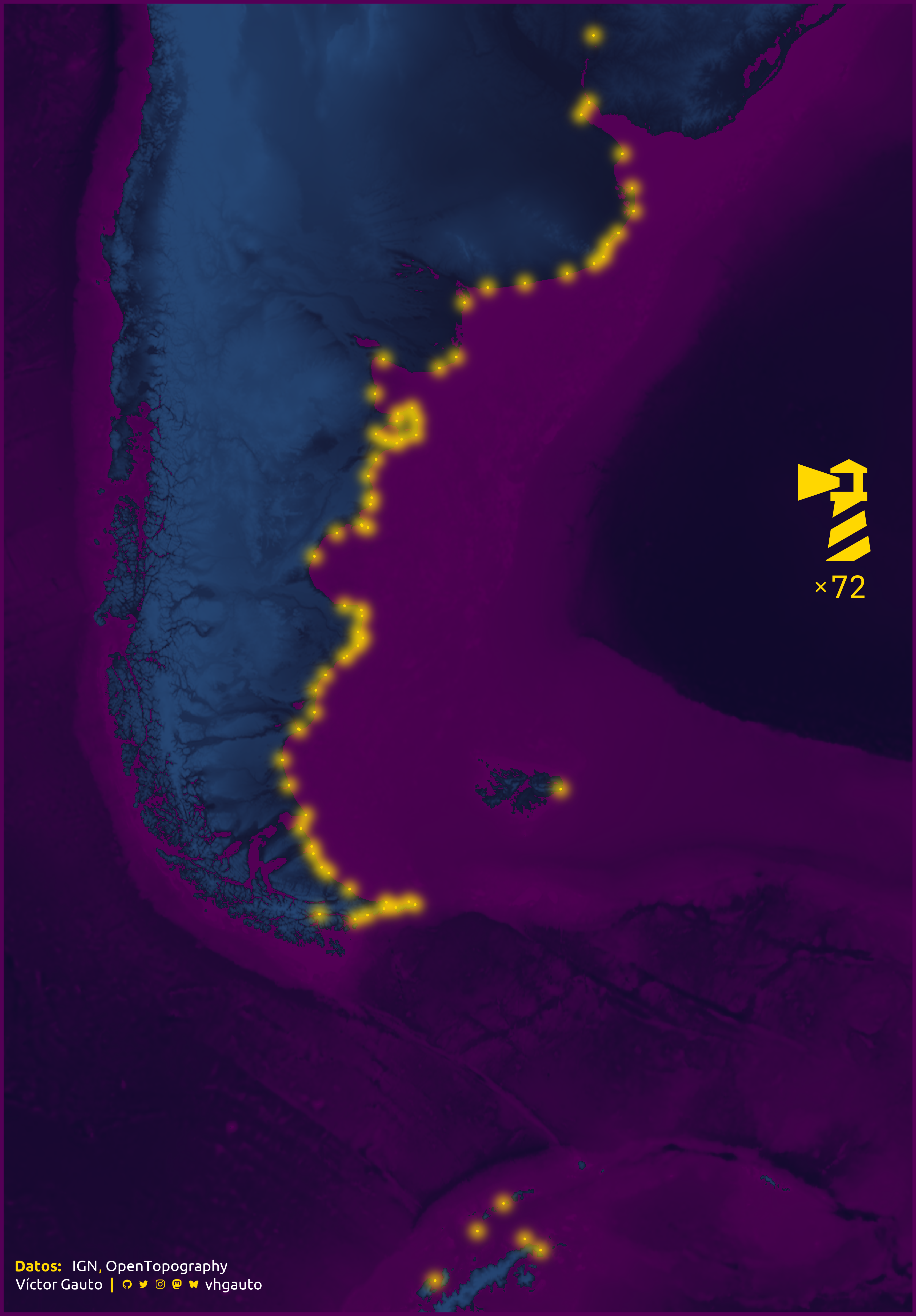
library(tidyverse)Faros en las costas de Argentina, con topografía como mapa base.
library(terra)
library(ggtext)
library(showtext)
library(glue)
library(ggfx)
library(tidyverse)c_arriba <- c("#131631", "#264775")
c_abajo <- c("#100A2C", "#540056")
c1 <- "white"
c2 <- "gold"
font_add(
family = "ubuntu",
regular = "././fuente/Ubuntu-Regular.ttf",
bold = "././fuente/Ubuntu-Bold.ttf",
italic = "././fuente/Ubuntu-Italic.ttf"
)
font_add(
family = "jet",
regular = "././fuente/JetBrainsMonoNLNerdFontMono-Regular.ttf"
)
showtext_auto()
showtext_opts(dpi = 300)fuente <- glue(
"<b>Datos: </b> <span style='color:{c1};'>IGN</span>,
</b> <span style='color:{c1};'>OpenTopography</span>"
)
autor <- glue("<span style='color:{c1};'>Víctor Gauto</span>")
icon_twitter <- glue(
"<span style='font-family:jet;'></span>"
)
icon_instagram <- glue(
"<span style='font-family:jet;'></span>"
)
icon_github <- glue(
"<span style='font-family:jet;'></span>"
)
icon_mastodon <- glue(
"<span style='font-family:jet;'>󰫑</span>"
)
icon_bluesky <- glue(
"<span style='font-family:jet;'></span>"
)
usuario <- glue("<span style='color:{c1};'>vhgauto</span>")
sep <- glue("**|**")
mi_caption <- glue(
"{fuente}<br>{autor} {sep} <b>{icon_github} {icon_twitter} ",
"{icon_instagram} {icon_mastodon} {icon_bluesky}</b> {usuario}"
)Vector de faros en las costas de Argentina, descargado del Instituto Geográfico Nacional (Hidrografía y oceanografía / Ayuda a la navegación / Punto / Faro).
faro <- vect(
  "argentina/vectores/ayuda_a_la_navegacion_BC050.json"
) |>
project("EPSG:5346")Incremento el contorno del vector de faros para la descarga del modelo digital de elevación.
e1 <- ext(faro)$xmin
e2 <- ext(faro)$xmax
e3 <- ext(faro)$ymin
e4 <- ext(faro)$ymax

faro_bb_elev <- vect(
  ext(e1-8e5, e2+8e5, e3-1e5, e4+1e5), "EPSG:5346"
)
faro_bb_elev_sf <- faro_bb_elev |>
  sf::st_as_sf()
Descarga de datos de elevación.
ele_arg <- elevatr::get_elev_raster(
  locations = faro_bb_elev_sf,
  z = 5,
  clip = "locations"
) |>
  rast() |>
  project("EPSG:5346")

names(ele_arg) <- "altura"
Divido los datos por arriba y abajo del nivel de 0m, así aplico dos escalas de color.
arriba <- ele_arg
arriba[arriba<0] <- NA
Paleta de colores.
f_arriba <- colorRampPalette(c_arriba)
paleta_arriba <- f_arriba(length(cells(arriba)))
Convierto a tibble y agrego colores, de acuerdo a la altura.
arriba_tbl <- arriba |>
  as.data.frame(xy = TRUE) |>
  tibble() |>
  arrange(altura) |>
  mutate(n = row_number()) |>
  mutate(color = paleta_arriba[n])
Abajo, remuevo todo lo mayor a 0m.
abajo <- ele_arg
abajo[abajo>0] <- NA
Paleta de colores.
f_abajo <- colorRampPalette(c_abajo)
paleta_abajo <- f_abajo(length(cells(abajo)))
Convierto a tibble y agrego colores, de acuerdo a la altura.
abajo_tbl <- abajo |>
  as.data.frame(xy = TRUE) |>
  tibble() |>
  arrange(altura) |>
  mutate(n = row_number()) |>
  mutate(color = paleta_abajo[n])
Obtengo las coordenadas de los faros.
faro_tbl <- as.data.frame(faro, geom = "XY") |>
tibble()Relación de aspecto del mapa.
ext_bb <- ext(faro_bb_elev)
asp <- (ext_bb$ymax - ext_bb$ymin)/(ext_bb$xmax - ext_bb$xmin)
Tamaño del mapa, en centímetros.
ancho <- 30
alto <- ancho*asp
Íconos y subtítulo.
faro_icon <- glue(
"<span style='font-family:jet;font-size:150px;'>󰨀</span>"
)
equis_icon <- ""
mi_subtitle <- glue(
"{faro_icon}<br>",
"{equis_icon}{length(faro)}"
)Figura.
g <- ggplot() +
  # abajo
  geom_raster(data = abajo_tbl, aes(x, y, fill = color)) +
  # arriba
  geom_raster(data = arriba_tbl, aes(x, y, fill = color)) +
  # faros
  with_blur(
    geom_point(
      data = faro_tbl, aes(x, y), color = c2, size = 6, alpha = 1
    ),
    sigma = 20
  ) +
  geom_point(
    data = faro_tbl, aes(x, y), color = c2, size = .5, alpha = 1
  ) +
  # subtítulo
  annotate(
    geom = "richtext", x = ext_bb$xmax*.98, y = ext_bb$ymin*1.8,
    label = mi_subtitle, family = "jet", color = c2, fill = NA,
    size = 10, label.color = NA, hjust = 1
  ) +
  # epígrafe
  annotate(
    geom = "richtext", x = ext_bb$xmin*1.01, y = ext_bb$ymin*1.02,
    label = mi_caption, family = "ubuntu", color = c2, fill = NA,
    size = 5, label.color = NA, hjust = 0, vjust = 0
  ) +
  # cuadro
  annotate(
    geom = "rect", xmin = ext_bb$xmin, xmax = ext_bb$xmax, ymin = ext_bb$ymin,
    ymax = ext_bb$ymax, color = c_abajo[2], linewidth = 3, fill = NA
  ) +
  scale_fill_identity() +
  coord_fixed(expand = FALSE) +
  theme_void()
Guardo la figura.
ggsave(
  plot = g,
  filename = "argentina/instalaciones/faros.png",
  width = ancho,
  height = alto,
  units = "cm"
)