Ocultar código
library(glue)
library(ggtext)
library(showtext)
library(terra)
library(tidyterra)
library(ggspatial)
library(patchwork)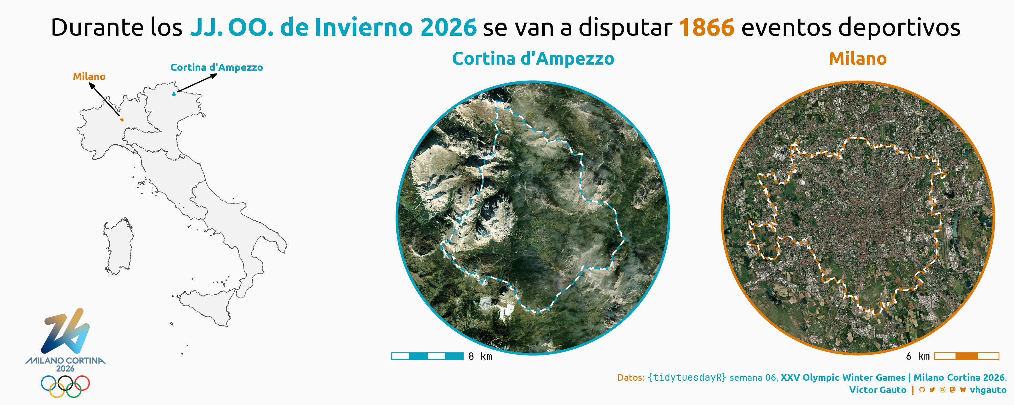
library(tidyverse)Mapas RGB de las ciudades en las que ocurren los JJ. OO. de Invierno 2026, Milano y Cortina.
library(glue)
library(ggtext)
library(showtext)
library(terra)
library(tidyterra)
library(ggspatial)
library(patchwork)
library(tidyverse)Colores.
c1 <- "#05a3bd"
c2 <- "#da7900"
c3 <- "white"
c4 <- "grey95"
c5 <- "grey30"
c6 <- "grey98"
Fuentes: Ubuntu y JetBrains Mono.
font_add(
  family = "ubuntu",
  regular = "././fuente/Ubuntu-Regular.ttf",
  bold = "././fuente/Ubuntu-Bold.ttf",
  italic = "././fuente/Ubuntu-Italic.ttf"
)

font_add(
  family = "jet",
  regular = "././fuente/JetBrainsMonoNLNerdFontMono-Regular.ttf"
)

showtext_auto()
showtext_opts(dpi = 300)fuente <- glue(
"Datos: <span style='color:{c1};'><span style='font-family:jet;'>",
"{{<b>tidytuesdayR</b>}}</span> semana 06, ",
"<b>XXV Olympic Winter Games | Milano Cortina 2026</b>.</span>"
)
autor <- glue("<span style='color:{c1};'>**Víctor Gauto**</span>")
icon_twitter <- glue("<span style='font-family:jet;'></span>")
icon_instagram <- glue("<span style='font-family:jet;'></span>")
icon_github <- glue("<span style='font-family:jet;'></span>")
icon_mastodon <- glue("<span style='font-family:jet;'>󰫑</span>")
icon_bsky <- glue("<span style='font-family:jet;'></span>")
usuario <- glue("<span style='color:{c1};'>**vhgauto**</span>")
sep <- glue("**|**")
mi_caption <- glue(
"{fuente}<br>{autor} {sep} {icon_github} {icon_twitter} {icon_instagram} ",
"{icon_mastodon} {icon_bsky} {usuario}"
)tuesdata <- tidytuesdayR::tt_load(2026, 06)
schedule <- tuesdata$scheduleMe interesa señalar las ciudades de los JJ.OO., Milano y Cortina, en un mapa de Italia, y mostrar mapas satelitales para cada una.
Creo un vector con el nombre de las ciudades, para obtener los datos y generar los mapas. Asigno colores, obtengo las coordenadas y creo vector.
ciudades <- c("Cortina d'Ampezzo", "Milano")

ciudades_col <- c(c1, c2)
ciudades_col <- set_names(ciudades_col, ciudades)

cortina <- c(12.137351, 46.538333)
milan <- c(9.19, 45.466944)

df <- data.frame(
  lon = c(12.137351, 9.19),
  lat = c(46.538333, 45.466944),
  ciudad = ciudades
)

p <- vect(df, geom = c("lon", "lat"), crs = "EPSG:4326")
Vectores de Italia y de las ciudades.
it4 <- rgeoboundaries::geoboundaries(country = "ITA", adm_lvl = 4) |>
  terra::vect()

it1 <- rgeoboundaries::geoboundaries(country = "ITA", adm_lvl = 1) |>
  terra::vect()

v <- it4[it4$shapeName %in% ciudades]
Función para generar un vector buffer circular alrededor de las ciudades.
f_bb <- function(X) {
  v <- v[v$shapeName == X]
  centro <- centroids(v)
  buffer(centro, width = width(v) * .8, quadsegs = 1000)
}
Función para obtener ráster RGB de los buffer de las ciudades.
f_rgb <- function(X) {
  b <- f_bb(X)

  maptiles::get_tiles(
    x = b,
    provider = "Esri.WorldImagery",
    crop = TRUE,
    zoom = 13
  ) |>
    mask(b)
}
Ejecuto para ambas ciudades y asigno nombres.
l_rgb <- map(ciudades, f_rgb)
l_rgb <- set_names(l_rgb, ciudades)Función para generar los mapas de cada ciudad.
f_gg <- function(X) {
  colorX <- if (X == "Milano") ciudades_col[2] else ciudades_col[1]
  locationX <- if (X == "Milano") "br" else "bl"

  ggplot() +
    geom_spatraster_rgb(
      data = l_rgb[[X]],
      maxcell = prod(dim(l_rgb[[X]]))
    ) +
    geom_spatvector(
      data = v[v$shapeName == X],
      fill = NA,
      color = colorX,
      linetype = 1,
      linewidth = .6
    ) +
    geom_spatvector(
      data = v[v$shapeName == X],
      fill = NA,
      color = c3,
      linetype = 2,
      linewidth = .6
    ) +
    geom_spatvector(
      data = f_bb(X),
      fill = NA,
      color = colorX,
      linewidth = 1
    ) +
    annotation_scale(
      location = locationX,
      bar_cols = c(c3, colorX),
      height = unit(.2, "cm"),
      line_col = colorX,
      text_family = "jet"
    ) +
    coord_sf(clip = "off") +
    labs(title = X) +
    theme_void(base_family = "ubuntu") +
    theme_sub_plot(
      title = element_text(
        hjust = .5,
        face = "bold",
        size = 15,
        color = colorX,
        margin = margin_auto(0)
      )
    )
}
Genero los mapas.
l_gg <- map(ciudades, f_gg)Mapa de Italia señalando las ciudades.
gg_it <- ggplot() +
  geom_spatvector(
    data = it1,
    fill = c4,
    color = c5,
    linewidth = .2
  ) +
  geom_spatvector(
    data = v,
    aes(fill = shapeName),
    color = NA,
    show.legend = FALSE
  ) +
  annotate(
    geom = "segment",
    x = I(c(.48, .23)),
    xend = I(c(.65, .1)),
    y = I(c(.92, .84)),
    yend = I(c(.98, .95)),
    arrow = arrow(angle = 20, length = unit(5, "pt"), type = "closed")
  ) +
  annotate(
    geom = "label",
    x = I(c(.65, .1)),
    y = I(c(.98, .95)),
    label = ciudades,
    fill = NA,
    border.color = NA,
    fontface = "bold",
    family = "ubuntu",
    hjust = .5,
    vjust = 0,
    color = ciudades_col,
    size = 3
  ) +
  coord_sf(clip = "off", expand = TRUE) +
  scale_fill_manual(
    values = ciudades_col
  ) +
  theme_void()
Logo de los JJ. OO. para incorporar a la figura.
logo <- "https://upload.wikimedia.org/wikipedia/commons/7/71/2026_Winter_Olympics_logo_%28Energy%29.svg"
logo_txt <- paste(readLines(logo), collapse = "\n")
Combino los mapas y agrego el logo.
g <- wrap_plots(
  list(gg_it, l_gg[[1]], l_gg[[2]]),
  nrow = 1
) +
  annotation_custom(
    ggsvg::svg_to_rasterGrob(logo_txt),
    xmin = I(-2),
    xmax = I(-2.3),
    ymin = I(.2),
    ymax = I(-.1)
  ) &
  plot_annotation(
    title = glue(
      "Durante los <b style='color:{c1};'>JJ. OO. de Invierno 2026</b> se van a disputar <b style='color:{c2};'>{nrow(schedule)}</b> eventos deportivos"
    ),
    caption = mi_caption,
    theme = theme(
      plot.title = element_markdown(
        family = "ubuntu",
        size = 21,
        hjust = .5,
        margin = margin_auto(10)
      ),
      plot.caption = element_markdown(
        family = "ubuntu",
        color = c2,
        size = 8,
        lineheight = 1.3,
        margin = margin(t = 5, b = 3)
      ),
      plot.background = element_rect(fill = c6, color = NA)
    )
  )
Guardo.
ggsave(
  plot = g,
  filename = "tidytuesday/2026/semana_06.png",
  width = 30,
  height = 12,
  units = "cm"
)