Ocultar código
library(glue)
library(ggtext)
library(showtext)
library(tidyverse)Requerimientos de agua y nutrientes para plantas comestibles.
library(glue)
library(ggtext)
library(showtext)
library(tidyverse)Colores.
c1 <- "#eaf3ff"
c2 <- "#1a318b"
c3 <- "#f9e0e8"
c4 <- "#9a153d"
c5 <- "#5a2364"
c6 <- "grey90"
c7 <- "grey10"
Fuentes: Ubuntu y JetBrains Mono.
font_add(
  family = "ubuntu",
  regular = "././fuente/Ubuntu-Regular.ttf",
  bold = "././fuente/Ubuntu-Bold.ttf",
  italic = "././fuente/Ubuntu-Italic.ttf"
)

font_add(
  family = "jet",
  regular = "././fuente/JetBrainsMonoNLNerdFontMono-Regular.ttf"
)

font_add_google("Marvel", bold.wt = 800)

showtext_auto()
showtext_opts(dpi = 300)fuente <- glue(
"Datos: <span style='color:{c2};'><span style='font-family:jet;'>",
"{{<b>tidytuesdayR</b>}}</span> semana 05<br>",
"<b>Edible Plant Database, GROW Observatory</b>.</span>"
)
autor <- glue("<span style='color:{c2};'>**Víctor Gauto**</span>")
icon_twitter <- glue("<span style='font-family:jet;'></span>")
icon_instagram <- glue("<span style='font-family:jet;'></span>")
icon_github <- glue("<span style='font-family:jet;'></span>")
icon_mastodon <- glue("<span style='font-family:jet;'>󰫑</span>")
icon_bsky <- glue("<span style='font-family:jet;'></span>")
usuario <- glue("<span style='color:{c2};'>**vhgauto**</span>")
sep <- glue("**|**")
mi_caption <- glue(
"{fuente}<br>{autor} {sep} {icon_github} {icon_twitter} {icon_instagram} ",
"{icon_mastodon} {icon_bsky} {usuario}"
)tuesdata <- tidytuesdayR::tt_load(2026, 05)
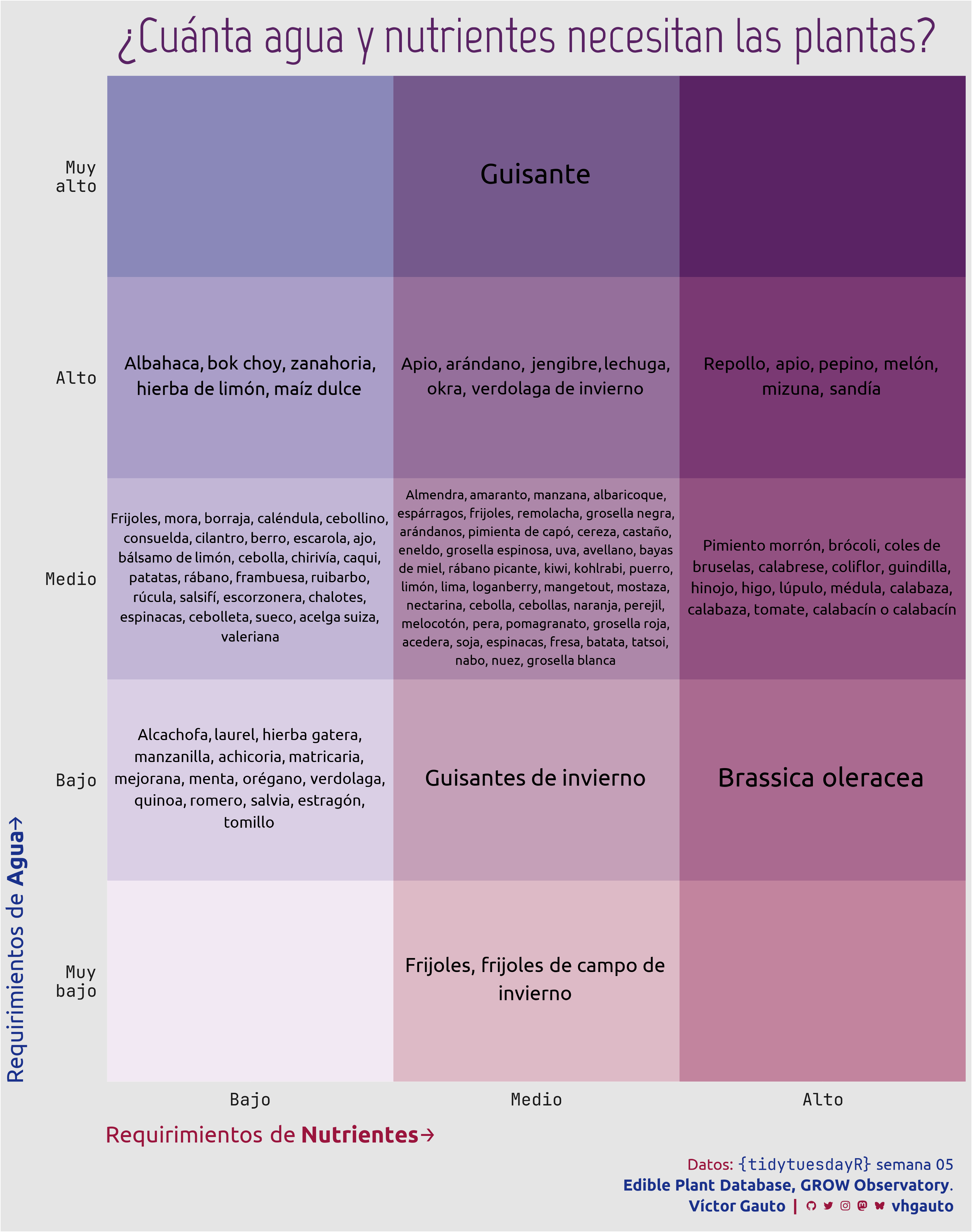
edible_plants <- tuesdata$edible_plantsMe interesa indicar las plantas asociadas a distintos niveles de agua y nutrientes.
Selecciono los requerimientos de agua y nutrientes, y sus traducciones.
orden_agua <- c("very low", "low", "medium", "high", "very high")
orden_agua_trad <- c("Muy bajo", "Bajo", "Medio", "Alto", "Muy alto") |>
  str_replace(" ", "\n")
orden_nutri <- c("low", "medium", "high")
orden_nutri_trad <- c("Bajo", "Medio", "Alto")
Selecciono los nombres de las plantas y la cantidad de agua y nutrientes requeridos.
ed <- edible_plants |>
  select(nombre = common_name, nutriente = nutrients, agua = water) |>
  mutate(across(c(agua, nutriente), tolower))
Creo un tibble con todas las combinaciones de agua y nutrientes. Agrego traducciones y combino con los nombres de las plantas.
ex <- expand_grid(
  agua_n = 1:5,
  nutriente_n = 1:3
)

d <- ex |>
  mutate(agua = orden_agua[agua_n]) |>
  mutate(nutriente = orden_nutri[nutriente_n]) |>
  full_join(ed, by = join_by(nutriente, agua)) |>
  drop_na(agua_n)
Obtengo el nombre de las plantas, sus traducciones y aplico formato. Calculo la cantidad de letras por cada combinación de nutrientes y agua, para luego asociar con el tamaño de letra.
Las traducciones se realizaron con el paquete {polyglotr}.
d_label <- d |>
  drop_na(nombre) |>
  mutate(nombre = tolower(nombre)) |>
  mutate(nombre = str_remove(nombre, " \\(.+\\)")) |>
  mutate(nombre = str_remove(nombre, " \\/.*")) |>
  distinct() |>
  arrange(nombre, agua_n) |>
  reframe(
    label = str_flatten_comma(nombre),
    .by = c(agua_n, nutriente_n)
  ) |>
  mutate(s = nchar(label)) |>
  mutate(
    label_es = map_chr(
      label,
      ~ polyglotr::mymemory_translate(.x, "es", "en")
    )
  ) |>
  mutate(label_es = tolower(label_es)) |>
  mutate(label_es = str_to_sentence(label_es)) |>
mutate(label_es = str_wrap(label_es, width = 50))Título y figura. El tamaño de texto en los cuadros es inversamente proporcional a la cantidad de letras.
mi_titulo <- "¿Cuánta agua y nutrientes necesitan las plantas?"
g <- ggplot(d, aes(nutriente_n, agua_n)) +
geom_tile(
data = ex,
aes(fill = agua_n),
show.legend = FALSE,
alpha = 1,
color = NA
) +
scale_fill_gradient(low = c1, high = c2) +
ggnewscale::new_scale(new_aes = "fill") +
geom_tile(
data = ex,
aes(fill = nutriente_n),
show.legend = FALSE,
alpha = .5,
color = NA,
linewidth = NA
) +
geom_textbox(
data = d_label,
aes(nutriente_n, agua_n, label = label_es, size = (1 / s)^(.15) * 10),
width = unit(9, "cm"),
lineheight = 1.4,
halign = .5,
valign = .5,
fill = NA,
box.color = NA,
family = "ubuntu"
) +
scale_x_continuous(breaks = 1:3, labels = orden_nutri_trad) +
scale_y_continuous(breaks = 1:5, labels = orden_agua_trad) +
scale_fill_gradient(low = c3, high = c4) +
scale_size_identity() +
labs(
x = glue(
"Requirimientos de **Nutrientes**",
"<span style='font-family:jet;'>→</span>"
),
y = glue(
"Requirimientos de **Agua**",
"<span style='font-family:jet;'>→</span>"
),
title = mi_titulo,
caption = mi_caption
) +
coord_cartesian(expand = FALSE) +
theme_gray(base_family = "ubuntu") +
theme_sub_plot(
background = element_rect(fill = c6),
title = element_markdown(
family = "Marvel",
size = 43,
color = c5,
margin = margin_auto(10)
),
caption = element_markdown(
color = c4,
size = 14,
lineheight = 1.3,
margin = margin_auto(10)
)
) +
theme_sub_panel(background = element_blank()) +
theme_sub_axis(
ticks = element_blank(),
text = element_text(
face = "bold",
color = c7,
family = "jet",
size = 15
)
) +
theme_sub_axis_bottom(
title = element_markdown(
size = 20,
color = c4,
hjust = 0,
margin = margin(t = 15)
),
text = element_text(margin = margin(t = 10))
) +
theme_sub_axis_left(
title = element_markdown(
size = 20,
color = c2,
hjust = 0,
margin = margin(r = 15)
),
text = element_text(margin = margin(r = 10))
)Guardo.
ggsave(
  plot = g,
  filename = "tidytuesday/2026/semana_05.png",
  width = 30,
  height = 38,
  units = "cm"
)