Ocultar código
library(glue)
library(ggtext)
library(showtext)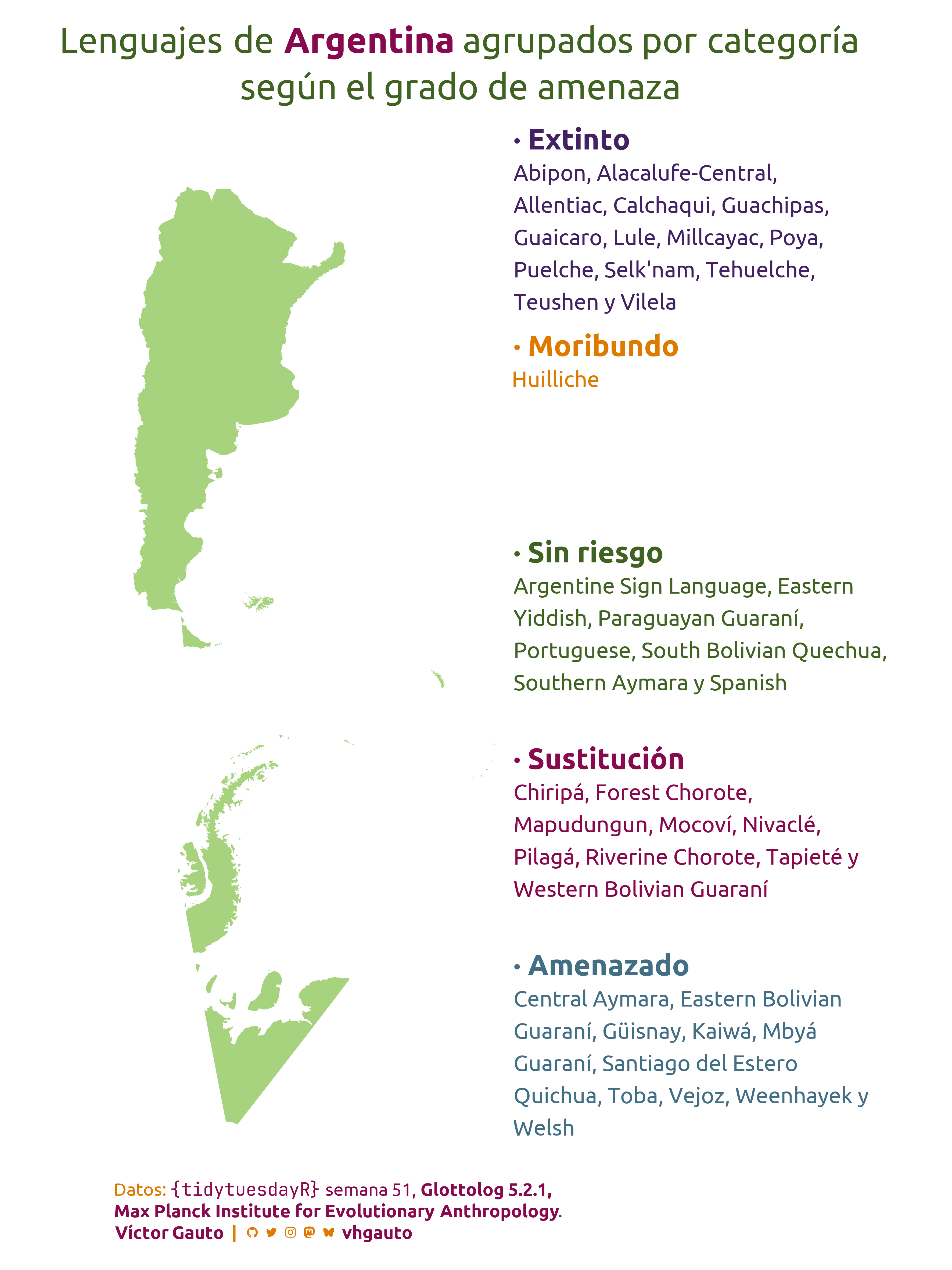
library(tidyverse)Lenguajes de Argentina agrupados por estado de amenaza.
library(glue)
library(ggtext)
library(showtext)
library(tidyverse)Colores.
col <- PrettyCols::prettycols("Dark")Fuentes: Ubuntu y JetBrains Mono.
font_add(
  family = "ubuntu",
  regular = "././fuente/Ubuntu-Regular.ttf",
  bold = "././fuente/Ubuntu-Bold.ttf",
  italic = "././fuente/Ubuntu-Italic.ttf"
)

font_add(
  family = "jet",
  regular = "././fuente/JetBrainsMonoNLNerdFontMono-Regular.ttf"
)

showtext_auto()
showtext_opts(dpi = 300)fuente <- glue(
"Datos: <span style='color:{col[5]};'><span style='font-family:jet;'>",
"{{<b>tidytuesdayR</b>}}</span> semana 51, ",
"<b>Glottolog 5.2.1,<br>Max Planck Institute for Evolutionary
Anthropology</b>.</span>"
)
autor <- glue("<span style='color:{col[5]};'>**Víctor Gauto**</span>")
icon_twitter <- glue("<span style='font-family:jet;'></span>")
icon_instagram <- glue("<span style='font-family:jet;'></span>")
icon_github <- glue("<span style='font-family:jet;'></span>")
icon_mastodon <- glue("<span style='font-family:jet;'>󰫑</span>")
icon_bsky <- glue("<span style='font-family:jet;'></span>")
usuario <- glue("<span style='color:{col[5]};'>**vhgauto**</span>")
sep <- glue("**|**")
mi_caption <- glue(
"{fuente}<br>{autor} {sep} {icon_github} {icon_twitter} {icon_instagram} ",
"{icon_mastodon} {icon_bsky} {usuario}"
)tuesdata <- tidytuesdayR::tt_load(2025, 51)
endangered_status <- tuesdata$endangered_status
families <- tuesdata$families
languages <- tuesdata$languagesMe interesan los lenguajes presentes en Argentina.
Leo vector bicontinental de Argentina, sin divisiones internas.
arg <- terra::vect("argentina/vectores/arg_bicontinental.gpkg")Expando los países presentes y filtro por Argentina, agrupando los lenguajes de acuerdo con la categoría de riesgo.
d <- inner_join(languages, endangered_status, by = join_by(id)) |>
  select(name, status_label, countries) |>
  separate_longer_delim(cols = countries, delim = ";") |>
  filter(countries == "AR") |>
  arrange(status_label, name) |>
  reframe(
    label = str_flatten_comma(name, last = " y "),
    .by = status_label
  ) |>
  mutate(label = str_wrap(label, 35))
Agrego la traducción de las categorías y la posición vertical del texto.
estados <- unique(d$status_label)
estados_trad <- c(
  "Extinto",
  "Moribundo",
  "Sin riesgo",
  "Sustitución",
  "Amenazado"
)

estados_trad <- set_names(estados_trad, estados)
l <- length(estados_trad)

d <- d |>
  mutate(estados_etq = estados_trad[status_label]) |>
mutate(y = seq(1, 0, length.out = l + 1)[1:l])Título y figura.
mi_titulo <- glue(
  "Lenguajes de <b style='color: {col[5]}'>Argentina</b> agrupados por
  categoría<br>según el grado de amenaza"
)

g <- ggplot() +
  tidyterra::geom_spatvector(
    data = arg,
    fill = scales::col_lighter(col[4], 40),
    color = NA
  ) +
  geom_text(
    data = d,
    aes(
      x = I(1),
      y = I(y),
      label = paste0("· ", estados_etq),
      color = estados_etq
    ),
    hjust = 0,
    size = 26,
    fontface = "bold",
    size.unit = "pt",
    family = "ubuntu",
    show.legend = FALSE
  ) +
  geom_text(
    data = d,
    aes(x = I(1), y = I(y - .025), label = label, color = estados_etq),
    hjust = 0,
    vjust = 1,
    size = 20,
    size.unit = "pt",
    family = "ubuntu",
    show.legend = FALSE
  ) +
  scale_color_manual(values = col) +
  coord_sf(clip = "off", expand = TRUE) +
  labs(title = mi_titulo, caption = mi_caption) +
  theme_void(base_family = "ubuntu", base_size = 20) +
  theme_sub_plot(
    background = element_rect(fill = "white"),
    margin = margin(l = -290, t = 25, b = 25),
    title = element_markdown(
      color = col[4],
      size = rel(1.6),
      hjust = .5,
      lineheight = 1.3,
      margin = margin(b = 30, l = 265)
    ),
    caption = element_markdown(color = col[3], hjust = 0, lineheight = 1.2)
  )
Guardo.
ggsave(
  plot = g,
  filename = "tidytuesday/2025/semana_51.png",
  width = 30,
  height = 40,
  units = "cm"
)